Case study: Hydrophobicity vs. protein length

View as Movie       BeanShell script along with data (zipped)

Keywords:

computable sequence properties, visualisations (built in and generic), correlation of numerical features

Initial situation:

Assume we want to analyse the membrane proteins of E.coli. Let’s further assume that we have a list of the membrane proteins derived, for example, from using  TMHMM (Krogh et al., 2001) (defining all proteins with more than 6 trans-membrane regions as membrane proteins). The other remaining proteins are simply defined as “lysate” proteins.

Questions:

• Is there any relationship between protein length and hydrophobicity i.e. between the GRAVY value (grand average hydrophobicity score) and protein length? Answer this question for the whole genome, membrane and lysate proteins only.

Data:

We have 3 multi FASTA files with amino acid sequences prepared:

Data file	Content
membrane.fasta	contains all membrane proteins of E.coli (all proteins with more than 6 membrane spanning regions predicted by TMHMM 2.0)
fullgenome.fasta	all proteins of E.coli
lysate.fasta	all proteins but without the membrane proteins as defined above.

Steps

Step 1: Data import

Simply import all three datasets to PROMPT by using the FASTA import feature. Choose “Import -> FASTA -> File” from PROMPT's menu and choose “protein” as sequence type in the following dialog.

Step 2: Analysis & Results

In this example we analyse whether the hydrophobicity of membrane proteins (GRAVY) correlates with protein length. First we  select the membrane.fasta object in the Input area. You can select an entry by simply clicking on it. To select more than one entry or to deselect entries keep the control-key pressed while clicking at the entries. Now choose from the PROMPT menu
"Analyse -> Computable sequence properties -> Length vs. Hydrophobicity".
This will show up as a new entry in the result list. This entry contains hydrophobicity and protein length for each protein. To visualise, just select this result entry and use the right mouse click to view the context menu. Use the “Visualize” Menu to run a simple scatter plot (Fig 1A).

 It is possible to compare any numeric features with the “Analyse -> Generic Annotations” option. Select again the membrane.fasta object in the Input area but choose now the option
“Analyse -> Generic Annotations -> Compare annotations within 1 set -> Numeric feature correlation”.
In the following dialog choose the two numeric variables that you want to analyze i.e. here we choose “length” and “HydrophobcityAvg”. The generic correlation returns two  results: CorNumeric1:statvalues and CorNumeric1:datapairs.

The first result CorNumeric1:statvalues contains the Pearson correlation value, Pearson correlation test p-value and other statistical values. The lower the p-value of the Pearson correlation test, the less likely it is that the observed correlation is by random. To view these values double-click at the CorNumeric1:statvalues entry or use the context popup menu and choose Show data.

Table 1. Results of the correlation test on protein length against hydrophobicity of lysate proteins. The first 2 rows show the Pearson correlation coefficient and the p-value of the correlation test. Additionally the mean, standard deviation and median as well as minimum and maximum of  the length and hydrophobicity values are provided.

FIELD	VALUE
Pearson_correlation	cor -0.6911572
Pearson_correlation_test_pvalue	2.82E-54
setA_Description	"length"
setB_Description	"HydrophobicityAvg"
setA_mean	458.8418
setA_std	148.8976
setA_median	438
setA_min	207
setA_max	1120
setB_mean	0.763398
setB_std	0.226708
setB_median	0.810462
setB_min	-0.03125
setB_max	1.185057

To reproduce the figure below right click on the CorNumeric1:datapairs and choose your desired plotting type.

Tip: Click at the figures below to enlarge them.

1A. Membrane proteins only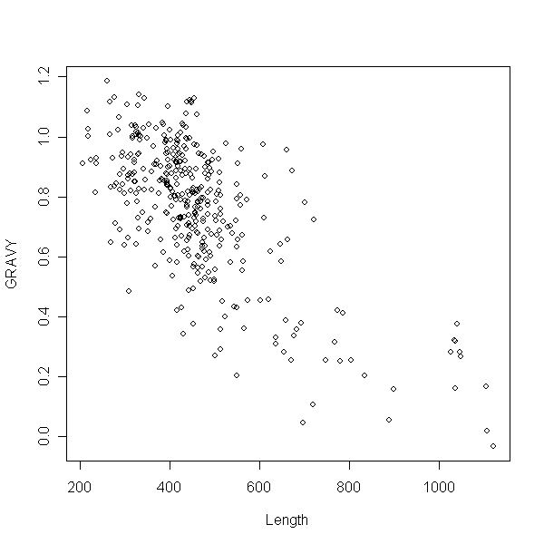

1B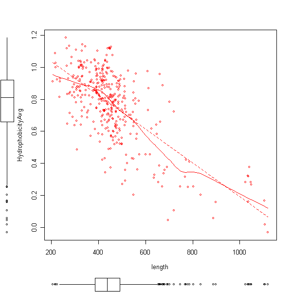

Figure 1 A and B: Length of membrane proteins against hydrophobicity (GRAVY). Figure B shows additionally a linear regression line (solid) and a local polynomial loess fitting (dotted line). The generic correlation tests shows a Pearson coefficient of -0.69 with a p-value of 2.8E-54.  The blue scatter plot was done with the default R plot method, the red plot uses the car-scatterplot R library.

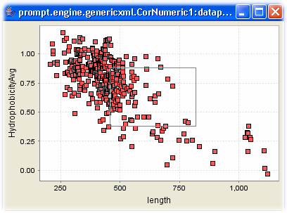
Additionally PROMPT provides interactive figures that allow one to zoom in and out. Furthermore the actual points can be identified and the accurate figures are shown as tooltips, as seen in Figure 1C.

1C. Interactive scatterplot Figure 1C. Protein length vs. hydrophobicity of lysate proteins. By pressing the left mouse button and keeping it pressed, you can define an area that shall be zoomed in or out.

We can repeat this for lysate proteins (Figure 2A) and all proteins (Figure 2B) of E.coli.
 

2A. Lysate proteins only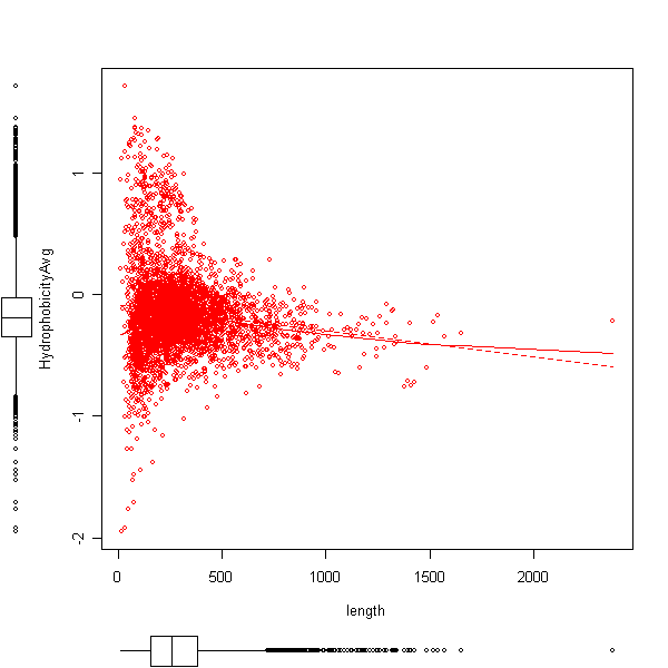

2B. Full genome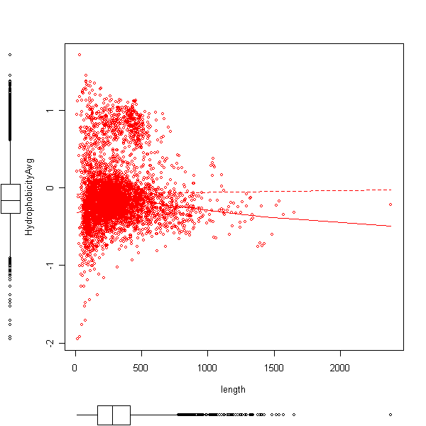

Figure 2 Length against hydrophobicity (GRAVY).
A) lysate proteins only, Pearson correlation -0.12 with p-value 1.2E-14
B) all proteins of E.coli, Pearson correlation 0.012 with p-value 0.43

Bottom line of this experiment: Longer membrane proteins tend to be less hydrophobic.

Summary:

• PROMPT can analyse the correlation between any numerical features
• In addition to correlation coefficients like Pearson's correlation, the significance of the observed correlation is computed (here with a Pearson correlation test)
• The graphical plots allow immediate visualisations and further analysis
• As shown in the external data example it is possible to use this type of analysis on any numerical external data.

More:

Start PROMPT, Download PROMPT or sign up to the Community Mailing List

Previous case study: Comparison of isoelectric point distributions

Back to the Case studies Overview

Next case study: Protein abundance analysis in yeast