
Case study: Protein abundance in yeast
View as Movie  BeanShell
script along with data (zipped)
BeanShell
script along with data (zipped) 
Keywords:
External data usage, Generic XML, Data Import/Export, Numeric correlation & comparisonInitial situation:
We have measured protein abundance data in yeast and want to analyse if abundance correlates with protein weight, mRNA expression or other numeric factors.
Questions:
- Does protein abundance correlate with mRNA expression levels?
- If there is a correlation and how strong is it, e.g. what is the Pearson correlation coefficient?
- How significant is the correlation?
- What is the probability that the observed correlation due to random noise?
- Are essential proteins more abundant in the cell?
Data:
We are using publicly available yeast protein abundance data (Ghaemmaghami S. et al. 2003 Nature) and steady-state mRNA expression levels of yeast proteins (Holstege, et al. 1998, Cell) (links). We formatted the original data as tab-delimited text files which PROMPT can import immediately. The format of PROMPT's tab-delimited files or PROMPT's generic XML format is described along with the descriptions of PROMPT's import methods Import-TXT and Import-XML.
Data file |
Content |
| mRNAexpr.txt | Steady-state mRNA expression levels |
| abd_all.txt | Protein abundance for all yeast proteins used in this study. The tab delimited text file contains the protein abundance in its original form and logarithmized to the base of 2. |
| abd_essential.txt | Protein abundance only for essential proteins in yeast |
| yeast.fasta | S.cerevisae protein sequences as multiple fasta file |
Steps
Step 1: Data import
Simply import all datasets to PROMPT by using the tab-delimited text import feature. Choose “Import -> TAB-Delimited TEXT file” from PROMPT's menu and select the files.
Step 2: Analysis & Results
Let's first of all analyse the correlation between mRNA expression levels and protein abundance:
Select the mRNAexpr input and the abd_all input and choose
Analyse -> Generic Annotations -> Compare annotation between 2 sets -> Numeric feature correlation
As the abd_all.txt input contains the original abundance values as well as the logarithmized abundance values you are asked which data you want to use. Select the property abundance that represents the non-logarithmized original data.
You'll get 2 results of a numeric correlation analysis. The first result named CorNumeric:statvalues contain the statistical values and results of the correlation test. The second result named CorNumeric:datapairs contains the datapairs and can be used to create a scatterplot. To view such a plot select the datapairs result and use the right mouse click to open a context-sensitive popup menu. In the popup menu select the CorrelationNumeric plot type. This is one of the static R plots that allow one to use logarithmic axis scales that are appropriate here.
Tip: Click at the figure to enlarge.
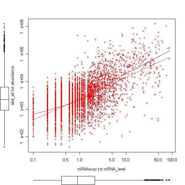
Note: A scatter plot visualisation with boxplots along the axes needs the additional R package car. Installation instructions can be found here.
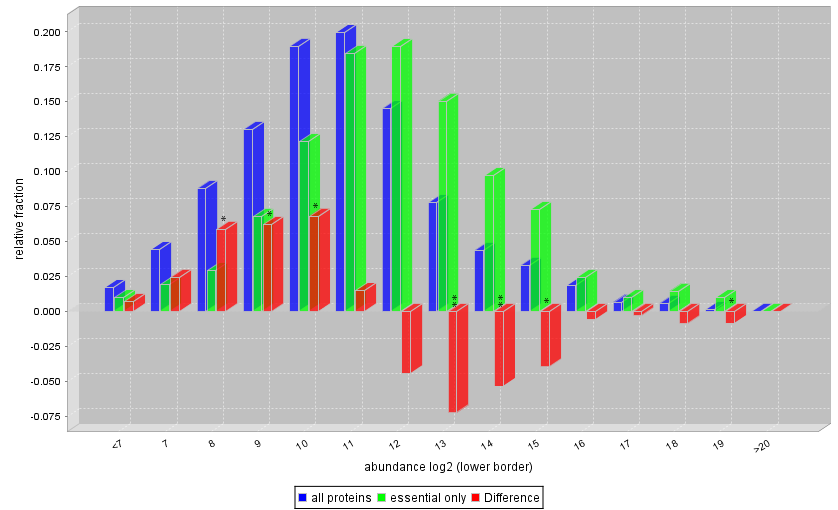
Our second question is are essential proteins more abundant? Let's see how the
molecule copy number differ between essential and all proteins.
Select the inputs abd_all.txt and abd_essential.txt. To run a numeric distribution comparison choose from PROMPT's menu
Analyse -> Generic Annotations -> Compare annotation between 2 sets -> Numeric feature comparison
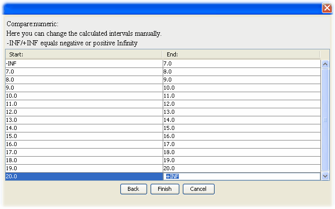
You are asked which numeric properties you want to compare. As both datasets contain logarithmized abundance values already choose "abundance_lg2". In the following binning wizard choose the following options:

Summary:
- The major analyses of PROMPT can be used with any generic data
- PROMPT allows one compare any numeric distributions and nominal categories independently of the origin or semantic of the external data.
- The binning of the histogram can be comfortably adjusted to one's own needs.
- External data can be imported immediately by a variety of ways e.g. by tab-delimited text files, PROMPT's generic XML format or using existing WEKA arff Files.
More:
Start PROMPT, Download PROMPT or sign up to the Community Mailing List
Previous case study: |
Back to the Case studies Overview |
Next case study: Fold enrichment in GroEL substrates |